Kaggle competition: Porto Seguro’s Safe Driver Prediction

Predicting if a driver will file an insurance claim.

The Jupyter notebook can be accessed here

Introduction to Kaggle competition

Nothing ruins the thrill of buying a brand new car more quickly than seeing your new insurance bill. The sting’s even more painful when you know you’re a good driver. It doesn’t seem fair that you have to pay so much if you’ve been cautious on the road for years.

Porto Seguro, one of Brazil’s largest auto and homeowner insurance companies, completely agrees. Inaccuracies in car insurance company’s claim predictions raise the cost of insurance for good drivers and reduce the price for bad ones.

In this competition, you’re challenged to build a model that predicts the probability that a driver will initiate an auto insurance claim in the next year. While Porto Seguro has used machine learning for the past 20 years, they’re looking to Kaggle’s machine learning community to explore new, more powerful methods. A more accurate prediction will allow them to further tailor their prices, and hopefully make auto insurance coverage more accessible to more drivers.

Seperating features

The dataset includes numerical, categorical and binary features. The numerical features consist of ordinal and float values. Each feature type needs to be treated separately, so first of all we can create three lists of columns for the three feature types.

I use the following code to separate the features based on their column names.

# separate col names into categories
cols = df.columns
num_feats, cat_feats, bin_feats = [], [], []

for col in cols:
    if col == 'id' or col == 'target':
        pass
    elif '_cat' in col:
        cat_feats.append(col)
    elif '_bin' in col:
        bin_feats.append(col)
    else:
        num_feats.append(col)

print('--- Numerical features --- : ', '\n', num_feats, '\n')
print('--- Categorical features --- : ', '\n', cat_feats, '\n')
print('--- Binary features --- : ', '\n', bin_feats, '\n')

The features are separated as follows:

— Numerical features — :
[‘ps_ind_01’, ‘ps_ind_03’, ‘ps_ind_14’, ‘ps_ind_15’, ‘ps_reg_01’, ‘ps_reg_02’, ‘ps_reg_03’, ‘ps_car_11’, ‘ps_car_12’, ‘ps_car_13’, ‘ps_car_14’, ‘ps_car_15’, ‘ps_calc_01’, ‘ps_calc_02’, ‘ps_calc_03’, ‘ps_calc_04’, ‘ps_calc_05’, ‘ps_calc_06’, ‘ps_calc_07’, ‘ps_calc_08’, ‘ps_calc_09’, ‘ps_calc_10’, ‘ps_calc_11’, ‘ps_calc_12’, ‘ps_calc_13’, ‘ps_calc_14’]

— Categorical features — :
[‘ps_ind_02_cat’, ‘ps_ind_04_cat’, ‘ps_ind_05_cat’, ‘ps_car_01_cat’, ‘ps_car_02_cat’, ‘ps_car_03_cat’, ‘ps_car_04_cat’, ‘ps_car_05_cat’, ‘ps_car_06_cat’, ‘ps_car_07_cat’, ‘ps_car_08_cat’, ‘ps_car_09_cat’, ‘ps_car_10_cat’, ‘ps_car_11_cat’]

— Binary features — :
[‘ps_ind_06_bin’, ‘ps_ind_07_bin’, ‘ps_ind_08_bin’, ‘ps_ind_09_bin’, ‘ps_ind_10_bin’, ‘ps_ind_11_bin’, ‘ps_ind_12_bin’, ‘ps_ind_13_bin’, ‘ps_ind_16_bin’, ‘ps_ind_17_bin’, ‘ps_ind_18_bin’, ‘ps_calc_15_bin’, ‘ps_calc_16_bin’, ‘ps_calc_17_bin’, ‘ps_calc_18_bin’, ‘ps_calc_19_bin’, ‘ps_calc_20_bin’]

Data cleansing

The next step is to check how many missing values there are for each feature type. As a general rule, I like to eliminate features where more than one half of the values are missing.

# Although it uses more memory, I prefer to create a new copy of the dataframe for each section
df_cleaned = df.copy()

# I will also create copies for the feature lists
num_feats_cleaned = num_feats.copy()
cat_feats_cleaned = cat_feats.copy()
bin_feats_cleaned = bin_feats.copy()

Numerical features

Let’s check for missing values (-1) in the numerical feature columns.

# I would like to eliminate any columns that consist of more than one half missing values (-1)
num_many_missing = df_cleaned[num_feats_cleaned][df == -1].count() / len(df) > 0.50 # more than 50% missing values
num_many_missing = num_many_missing.index[num_many_missing == True].tolist()
print(num_many_missing)

No columns were returned. We can also have a look at exactly how many are missing in the applicable columns.

counts = df_cleaned[num_feats_cleaned][df == -1].count()
cols_with_missing = counts[counts.values > 0]
print('Column  ', 'Missing count  ', 'Missing ratio')
for col, count in zip(cols_with_missing.index, cols_with_missing.values):
    print(col, '  ', count, '  ', '{:.3f}'.format(count / len(df)))

Column Missing count Missing ratio ps_reg_03 107772 0.181 ps_car_11 5 0.000 ps_car_12 1 0.000 ps_car_14 42620 0.072

We can substitute the missing values with the applicable column mean. This will limit their impact on the results.

# The few missing values that remain will be substituted with the column mean
for col in num_feats_cleaned:
    df_cleaned[col][df_cleaned[col] == -1] = df_cleaned[col].mean()
# Check that no missing values remain
(df_cleaned[num_feats_cleaned] == -1).sum().sum()   # sums instances of true for each column and then sums across columns

We can be satisfied that no missing values remain.

Categorical features

I would like to eliminate any columns that consist of more than one-half missing values (-1). If features contain a relatively small proportion of missing values, these values can be converted to dummy variables and may be a useful part of the analysis.

cat_many_missing = df_cleaned[cat_feats_cleaned][df == -1].count() / len(df) > 0.5
cat_many_missing = cat_many_missing.index[cat_many_missing == True].tolist()
print(cat_many_missing)

Only one column is returned (‘ps_car_03_cat’).

# We can also have a look exactly how many are missing in the applicable columns
counts = df_cleaned[cat_feats_cleaned][df == -1].count()
cols_with_missing = counts[counts.values > 0]
print('Column  ', 'Missing count  ', 'Missing ratio')
for col, count in zip(cols_with_missing.index, cols_with_missing.values):
    print(col, '  ', count, '  ', '{:.3f}'.format(count / len(df)))

Column Missing count Missing ratio ps_ind_02_cat 216 0.000 ps_ind_04_cat 83 0.000 ps_ind_05_cat 5809 0.010 ps_car_01_cat 107 0.000 ps_car_02_cat 5 0.000 ps_car_03_cat 411231 0.691 ps_car_05_cat 266551 0.448 ps_car_07_cat 11489 0.019 ps_car_09_cat 569 0.001

Now I will remove the one column that I identified.

df_cleaned.drop(columns=cat_many_missing, inplace=True)

# The cat_feats list needs to be updated
for i in cat_many_missing: cat_feats_cleaned.remove(i)

Remaing missing values will be converted to dummy variables during the feature engineering stage.

Binary features

Let’s now check for missing values among the binary features.

bin_many_missing = df_cleaned[bin_feats_cleaned][df == -1].count() / len(df) > 0.5
bin_many_missing = bin_many_missing.index[bin_many_missing == True].tolist()
print(bin_many_missing)

No columns were returned where more than half of there values missing. Let’s just make sure that no values at all are missing for the binary features.

# Lets check for missing values, in case any exist
counts = df_cleaned[bin_feats_cleaned][df == -1].count()
cols_with_missing = counts[counts.values > 0]
cols_with_missing

Ok I am now satisfied that no missing values remain.

Exploratory data analysis

In this section, I will first explore the correlation between numerical features and then I will explore the correlation between each feature and the target variable to gain insight into feature importance.

Numerical features of float type

# First of all, we only want to select float values
df_float = df_cleaned.select_dtypes(['float64'])
df_corr = df_float.corr().abs()
# Setting a filter for values of 1 or less than 0.5
filter = (df_corr == 1) | (df_corr < 0.5)
# We can filter out values by setting them to 0
df_corr[filter] = 0
df_corr

f, ax = plt.subplots(figsize=(15, 10))
plt.title("\nPearson correlation of numeric features\n", size=24)
sns.heatmap(df_corr, annot=True, annot_kws={'size': 14},
            cmap=sns.diverging_palette(220, 20, n=11))

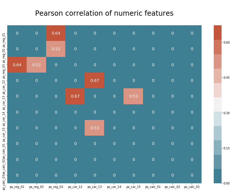
We can see that there are strong correlations between four pairs of features.

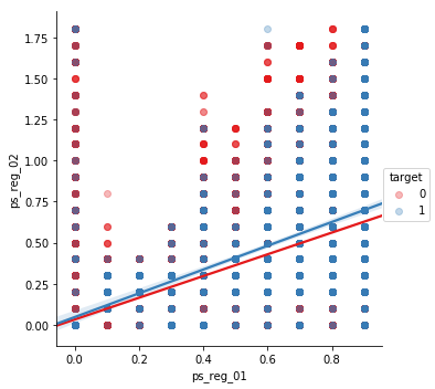
Let’s look at pair plots of the strongly correlated variables. This way we can gain insight into the linear correlations between the features.

sns.lmplot(x='ps_reg_01', y='ps_reg_02', data=df_cleaned.sample(frac=0.1), hue='target', palette='Set1', scatter_kws={'alpha':0.3})
plt.show()

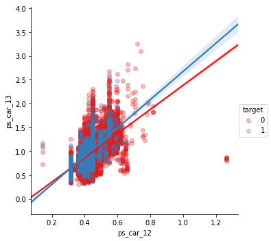
sns.lmplot(x='ps_car_12', y='ps_car_13', data=df_cleaned.sample(frac=0.1), hue='target', palette='Set1', scatter_kws={'alpha':0.3})
plt.show()

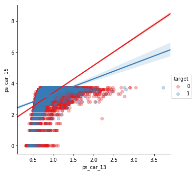
sns.lmplot(x='ps_car_13', y='ps_car_15', data=df_cleaned.sample(frac=0.1), hue='target', palette='Set1', scatter_kws={'alpha':0.3})
plt.show()

Numerical features of ordinal type Now let’s check how the ordinal features stack up against each other.

df_ordinal = df_cleaned[num_feats_cleaned].select_dtypes(include=['int'])
df_corr = df_ordinal.corr().abs()
filter = (df_corr == 1) | (df_corr < 0.1)
# We can filter out values by setting them to 0
df_corr[filter] = 0
df_corr

f, ax = plt.subplots(figsize=(15, 10))
plt.title("\nPearson correlation of orindal features\n", size=24)
sns.heatmap(df_corr, annot=True, annot_kws={'size': 14},
            cmap=sns.diverging_palette(220, 20, n=11))

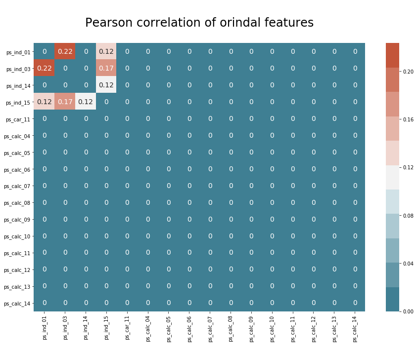
The correlations are very small, so not worthy of consideration.

Let’s now check the correlations between all numerical features and the target variables. We can use the pointbiserialr tool from scipy.stats to check the correlation between the numerical values of the features and the binary values of the target. The pointbiserialr method returns the correlation and the p-value. If the p-value is more than 0.05 for any given correlation, we cannot reject a null-hypothesis and should consider eliminating the feature, as it has a negligible impact on the target variable.

# check correlation between cols and target
num_weak_corr = []
for col in num_feats_cleaned:
    corr, p = pointbiserialr(df_cleaned[col], df_cleaned['target'])
    if p > .05:
        print(col.upper(), ' | Correlation: ', corr, '| P-value: ', p)
        num_weak_corr.append(col)

The following featuers are returned:

PS_CAR_11  | Correlation:  -0.00121335689622 | P-value:  0.349220144637
PS_CALC_01  | Correlation:  0.00178195465192 | P-value:  0.169200922734
PS_CALC_02  | Correlation:  0.00135968897833 | P-value:  0.294178988979
PS_CALC_03  | Correlation:  0.00190697359641 | P-value:  0.141229448762
PS_CALC_04  | Correlation:  3.27204551002e-05 | P-value:  0.979860521763
PS_CALC_05  | Correlation:  0.000770880136533 | P-value:  0.552022133573
PS_CALC_06  | Correlation:  8.18222597807e-05 | P-value:  0.949666387392
PS_CALC_07  | Correlation:  -0.000103476904853 | P-value:  0.936370675865
PS_CALC_08  | Correlation:  -0.00100585483842 | P-value:  0.43773988648
PS_CALC_09  | Correlation:  0.000718967584364 | P-value:  0.579111997695
PS_CALC_10  | Correlation:  0.00106083404448 | P-value:  0.413110667262
PS_CALC_11  | Correlation:  0.000371437394891 | P-value:  0.774446720276
PS_CALC_12  | Correlation:  -0.00113258539814 | P-value:  0.382233773313
PS_CALC_13  | Correlation:  -0.000446464531809 | P-value:  0.730510442941
PS_CALC_14  | Correlation:  0.00136227534312 | P-value:  0.2932615811

Categorical features

For checking correlation between the categorical features and the target variable, we can create a crosstab table using Pandas and apply the Chi-squared tool to determine a p-value. Once again, if the p-value is more than 0.05, then we could reject that feature.

cat_weak_corr = []
for col in cat_feats_cleaned:
    crosstab = pd.crosstab( df['target'], df_cleaned[col],  rownames = ['target'] , colnames =['feature'])
    chi2, p, dof, ex = chi2_contingency(crosstab, correction=False)
    if p > 0.05:
        print(col.upper(), ' | Chi2: ', chi2, ' | p-value: ', p)
        cat_weak_corr.append(col)

One feature is returned:

PS_CAR_10_CAT  | Chi2:  0.648974774486  | p-value:  0.722897825327

Binary features

We can do the same for the binary variables as we did for the categorical variables.

bin_weak_corr = []
for col in bin_feats_cleaned:
    crosstab = pd.crosstab( df['target'], df_cleaned[col],  rownames = ['target'] , colnames =['feature'])
    chi2, p, dof, ex = chi2_contingency(crosstab)
    if p > 0.05:
        print(col.upper(), ' | Chi2: ', chi2, ' | p-value: ', p)
        bin_weak_corr.append(col)

The following features are returned:

PS_IND_10_BIN  | Chi2:  1.49083915207  | p-value:  0.222086306306
PS_IND_11_BIN  | Chi2:  2.19212980726  | p-value:  0.138717387178
PS_IND_13_BIN  | Chi2:  3.18877595278  | p-value:  0.0741455110366
PS_CALC_15_BIN  | Chi2:  0.135285302885  | p-value:  0.713013790073
PS_CALC_16_BIN  | Chi2:  0.224798128543  | p-value:  0.635408055174
PS_CALC_17_BIN  | Chi2:  0.01544956754  | p-value:  0.901080685209
PS_CALC_18_BIN  | Chi2:  0.17519257769  | p-value:  0.675537637115
PS_CALC_19_BIN  | Chi2:  1.79054056273  | p-value:  0.180860314623
PS_CALC_20_BIN  | Chi2:  0.668511486963  | p-value:  0.413571052218

Using classification tools

Another approach is to use a classication tool - such as the random forest classifier - to determine the importance of each feature. We can achieve this by fitting a model and then calling the feature_importances method.

# Sets up a classifier and fits a model to all features of the dataset
clf = RandomForestClassifier(n_estimators=150, max_depth=8, min_samples_leaf=4, max_features=0.2, n_jobs=-1, random_state=0)
clf.fit(df_cleaned.drop(['id', 'target'],axis=1), df_cleaned['target'])
# We need a list of features as well
features = df_cleaned.drop(['id', 'target'],axis=1).columns.values
print("--- COMPLETE ---")

Using the following code from Anisotropic’s kernal (https://www.kaggle.com/arthurtok/interactive-porto-insights-a-plot-ly-tutorial), we can use Plotly to create a nice horizontal bar chart for visualising the ranking of most important features. (Make sure you install the Plotly extension of Jupyter lab by entering the following command in the terminal: jupyter labextension install @jupyterlab/plotly-extension)

x, y = (list(x) for x in zip(*sorted(zip(clf.feature_importances_, features),
                                                            reverse = False)))
trace2 = go.Bar(
    x=x ,
    y=y,
    marker=dict(
        color=x,
        colorscale = None,
        reversescale = True
    ),
    name='Random Forest Feature importance',
    orientation='h',
)

layout = dict(
    title='Ranking of most influential features',
     width = 900, height = 1500,
    yaxis=dict(
        showgrid=False,
        showline=False,
        showticklabels=True,
    ))

fig1 = go.Figure(data=[trace2])
fig1['layout'].update(layout)
py.iplot(fig1, filename='plots')

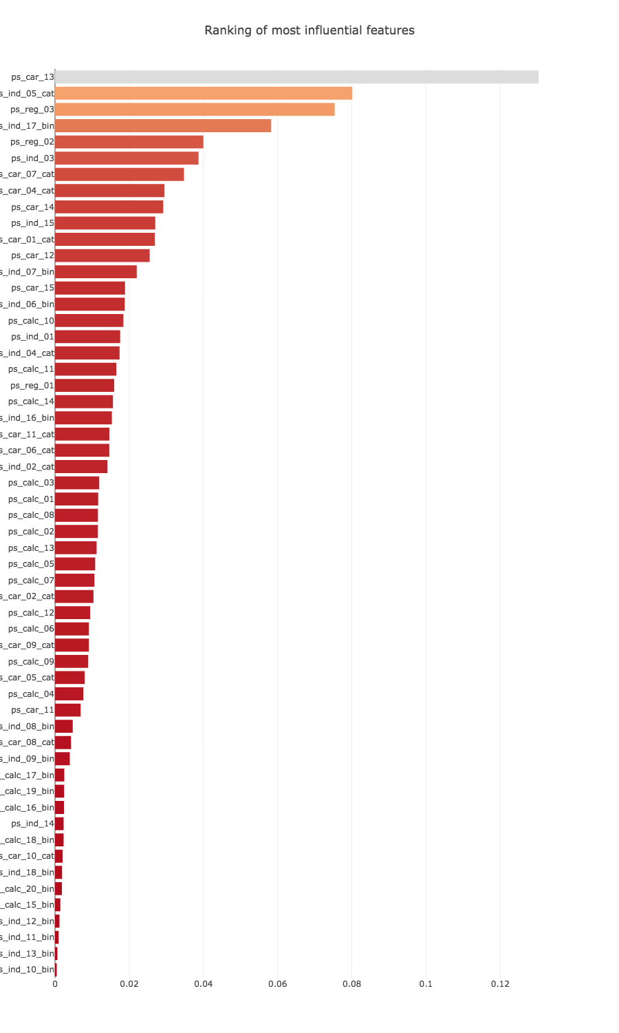
Feature selection

I would like to select only the features that have the greatest impact according to the graph above, with a combination of all features types.

feats_to_keep = ['ps_ind_06_bin',
                     'ps_car_15',
                     'ps_ind_07_bin',
                     'ps_car_12',
                     'ps_car_01_cat',
                     'ps_ind_15',
                     'ps_car_14',
                     'ps_car_04_cat',
                     'ps_car_07_cat',
                     'ps_ind_03',
                     'ps_reg_02',
                     'ps_ind_17_bin',
                     'ps_reg_03',
                     'ps_ind_05_cat',
                     'ps_car_13']

We need to separate the features out again, as we did at the start.

--- Numerical features --- :  
 ['ps_car_15', 'ps_car_12', 'ps_ind_15', 'ps_car_14', 'ps_ind_03', 'ps_reg_02', 'ps_reg_03', 'ps_car_13']

--- Categorical features --- :  
 ['ps_car_01_cat', 'ps_car_04_cat', 'ps_car_07_cat', 'ps_ind_05_cat']

--- Binary features --- :  
 ['ps_ind_06_bin', 'ps_ind_07_bin', 'ps_ind_17_bin']

Feature engineering

We still need to deal with the categorical variables because we cannot read them in as they are. We need to create dummy variables for each feature. This will greatly increase the number of features that we have, so I would like to minimize these features if I can.

We can check how many categories there are for each feature. This way we know which features are going to result in the most additional features after converting them to dummy variables.

df_engineered[cat_feats_to_keep].nunique()

ps_car_01_cat    13
ps_car_04_cat    10
ps_car_07_cat     3
ps_ind_05_cat     8
dtype: int64

Now we can use the Pandas get_dummies function to convert to dummy variables in new columns.

# convert cat feats to dummy variables (0s and 1s)
cat_dummy_df = pd.get_dummies(df_engineered[cat_feats_to_keep].astype(str))
# replacing original cat cols with new dummie cols
df_engineered = pd.concat([df_engineered, cat_dummy_df], axis=1).drop(columns=cat_feats_to_keep)

I now expect to see many more columns (features).

df_engineered.shape

(595212, 47)

Class balancing

Before going into feature scaling, I would like to check out the ratio of ones to zeros in the target variable. The reason I want to do this is because I already know that there is a very large class imbalance. We would not expect half of the people who are insured to lodge a claim.

df_engineered['target'].value_counts()

0    573518
1     21694
Name: target, dtype: int64

Sure enough, there are many more zeros. We can either over-sample (duplicate the training examples corresponding to the ones) or under-sample (remove training examples corresponding to the zeros).

Under-sampling from examples with a target of zero

I would like to select a sample that makes up half of the original length of the dataset.

df_zeros = df_engineered[df_engineered['target'] == 0]
df_zeros_sample = df_zeros.sample(n=int(rows / 2), random_state=42)
df_zeros_sample.reset_index(inplace=True, drop=True)

Over-sampling examples with a target of one

I will duplicate all of the examples corresponding to ones.

df_ones = df_engineered[df_engineered['target'] == 1]
# Adds duplicates of the ones set until half of the dataset is occupied
df_ones_dup = pd.DataFrame()
for i in range(int((rows / 2) / num_ones)):
    df_ones_dup = df_ones_dup.append(df_ones)

Combining examples into one dataset

Now I want to combine the two sample sets together to form one dataset of original length, where the ones and zeros are roughly balanced 1:1.

df_rebalanced = pd.concat([df_zeros_sample, df_ones_dup])
df_rebalanced = df_rebalanced.sample(frac=1).reset_index(drop=True)

Feature scaling

Scaling features tends to lead to a performance improvement with classification problems, so we will do it here.

df_scaled = df_rebalanced.copy()
df_scaled.drop(columns=['target', 'id'], inplace=True)
# Set up scaler and create a scaled input matrix
scaler = MinMaxScaler()
# MinMaxScalar outputs data as a numpy array (which is necessary for XGBoost)
X_scaled = scaler.fit_transform(df_scaled)

Training and Evaluation

Now we can split the data up into train and test sets, fit classification models to the train set and finally try to classify examples from the test set and observe the resulting accuracy and F1 scores.

X = X_scaled
# y needs to be converted to an array
y = df_rebalanced['target'].as_matrix()
# split up the data and target values
X_train, X_test, y_train, y_test = train_test_split(X, y, test_size=0.2)

models = []
models.append(('LogReg', LogisticRegression()))
models.append(('XGBoost', XGBClassifier()))

for name, model in models:
    print('\n++++++++++++++ {} ++++++++++++++\n'.format(name))

    # Train model
    print('\n--- Training model using {} ---'.format(name))
    model.fit(X_train, y_train)
    print('=== DONE ===\n')

    # Save model
    joblib.dump(model, '{}_model_trained.pkl'.format(name))

    # Make predictions on the test-set
    y_pred = model.predict(X_test)

    # Classification report
    report = classification_report(y_test, y_pred)
    print('\n', report, '\n')

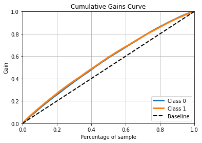
    # Plotting cumulative gains chart (lift curve)
    predicted_probas = LogReg_model.predict_proba(X_test)
    skplt.metrics.plot_cumulative_gain(y_test, predicted_probas)
    plt.show()

    print('======================================\n')

And here are the results that get printed out.

++++++++++++++ LogReg ++++++++++++++


--- Training model using LogReg ---
=== DONE ===


              precision    recall  f1-score   support

          0       0.59      0.67      0.62     59588
          1       0.59      0.50      0.54     56338

avg / total       0.59      0.59      0.58    115926

======================================


++++++++++++++ XGBoost ++++++++++++++


--- Training model using XGBoost ---
=== DONE ===


              precision    recall  f1-score   support

          0       0.60      0.67      0.63     59588
          1       0.60      0.52      0.56     56338

avg / total       0.60      0.60      0.60    115926

Conclusion

I know there is much room for improvement here. There are some excellent kernals for this competition that use novel techniques to drive up the gini score. I would like to go back over this project and apply new feature engineering techniques and optimise the hyperparameters of the XGBoost classifier. This is nice messy problem with a large variety of feature types and a heavily imbalanced dataset. All in all, a great competition for getting the hands dirty.